Palettes and Visualization
Note:This notebook includes interactive map visualizations using thegeemappackage. Additionally, you will likely need to installipykernelto utilize the interactive elements within a Jupyter Notebook. Thegeemapandipykernelpackages are not installed automatically withRadGEEToolboxsince they are optional dependencies focused on visualizations. If you have not already installed these packages, you can do so with:pip install geemap ipykernelAlternatively, using conda:
conda install conda-forge::geemap anaconda::ipykernelIf you do not install them, the map-based portions of this notebook will not work.
[1]:
import ee
import geemap
from RadGEEToolbox import LandsatCollection
from RadGEEToolbox import GetPalette
from RadGEEToolbox import VisParams
[ ]:
# Store name of Google Cloud Project assosiated with Earth Engine - replace with your project ID/name
PROJECT_ID = 'your-cloud-project-id'

# Attempt to initialize Earth Engine
try:
    ee.Initialize(project=PROJECT_ID)
    print("Earth Engine initialized successfully.")
except Exception as e:
    print("Initialization failed, attempting authentication...")
    try:
        ee.Authenticate()
        ee.Initialize(project=PROJECT_ID)
        print("Authentication and initialization successful.")
    except Exception as auth_error:
        print("Authentication failed. Error details:", auth_error)
Earth Engine initialized successfully.
RadGEEToolbox hosts two packages to help image visualization: 1) GetPalette and 2) VisParams
GetPalette has the get_palette() function which allows for easily getting the hex series for a variety of palettes
VisParams has the get_visualization_params() function which provides an alternative to visualization parameter dictionaries
[3]:
# Example getting the jet palette
# options: 'algae', 'dense', 'greens', 'haline', 'inferno', 'jet', 'matter', 'pubu', 'soft_blue_green_red', 'thermal', 'turbid', 'ylord'

jet = GetPalette.get_palette('jet')
print(jet)
['#00007F', '#002AFF', '#00D4FF', '#7FFF7F', '#FFD400', '#FF2A00', '#7F0000']
get_visualization_params() takes satellite, index, min_val, max_val, and palette as arguments
min_val, max_val, and palette are optional, however, as defaults are provided based on the satellite and index
providing optional values will override the defaults
Options for satellite: ‘Landsat’, ‘landsat’, ‘Sentinel2’, or ‘sentinel2’
Options for index: ‘TrueColor’, ‘NDVI’, ‘NDWI’, ‘halite’, ‘gypsum’, ‘LST’, ‘NDTI’, ‘KIVU’, or ‘2BDA’
Below is an example of how to define the visualization parameters for a true color landsat image and then printing what the vis_params dictionary looks like
[4]:
true_color_vis_params = VisParams.get_visualization_params(satellite='landsat', index='TrueColor')
print(true_color_vis_params)
{'min': 0, 'max': 30000, 'bands': ['SR_B4', 'SR_B3', 'SR_B2']}
Another example, this time defining the visualization parameters for a NDVI landsat image and printing the dictionary
[5]:
ndvi_vis_params = VisParams.get_visualization_params(satellite='landsat', index='NDVI')
print(ndvi_vis_params)
{'min': 0, 'max': 0.5, 'bands': ['ndvi'], 'palette': ['#f7fcf5', '#e5f5e0', '#c7e9c0', '#a1d99b', '#74c476', '#41ab5d', '#238b45', '#006d2c', '#00441b']}
Pulling it all together
Lets
Define a collection,
Process the collection for various products (ndwi, median, LST),
Get list of dates of images,
Visualize most recent image as true color and singeband products
[6]:
col = LandsatCollection('2023-06-01', '2023-07-30', [32, 33], 38, 20) # 1.
col = col.MosaicByDate # 1.
ndwi = col.ndwi # 2
LST = col.LST # 2
mean_temperature = LST.mean # 2
dates = col.dates # 3
print(dates) # 3
['2023-06-21', '2023-06-29', '2023-07-07', '2023-07-15']
True Color Visualization
[7]:
Map = geemap.Map(center=(40.7514, -111.9064), zoom=9)
Map.addLayer(col.image_grab(-1), vis_params=VisParams.get_visualization_params('Landsat', 'TrueColor'))
print('Date of displayed image:', col.dates[-1])
Map
Date of displayed image: 2023-07-15
[7]:
Example of True Color Map Output from Above Cell

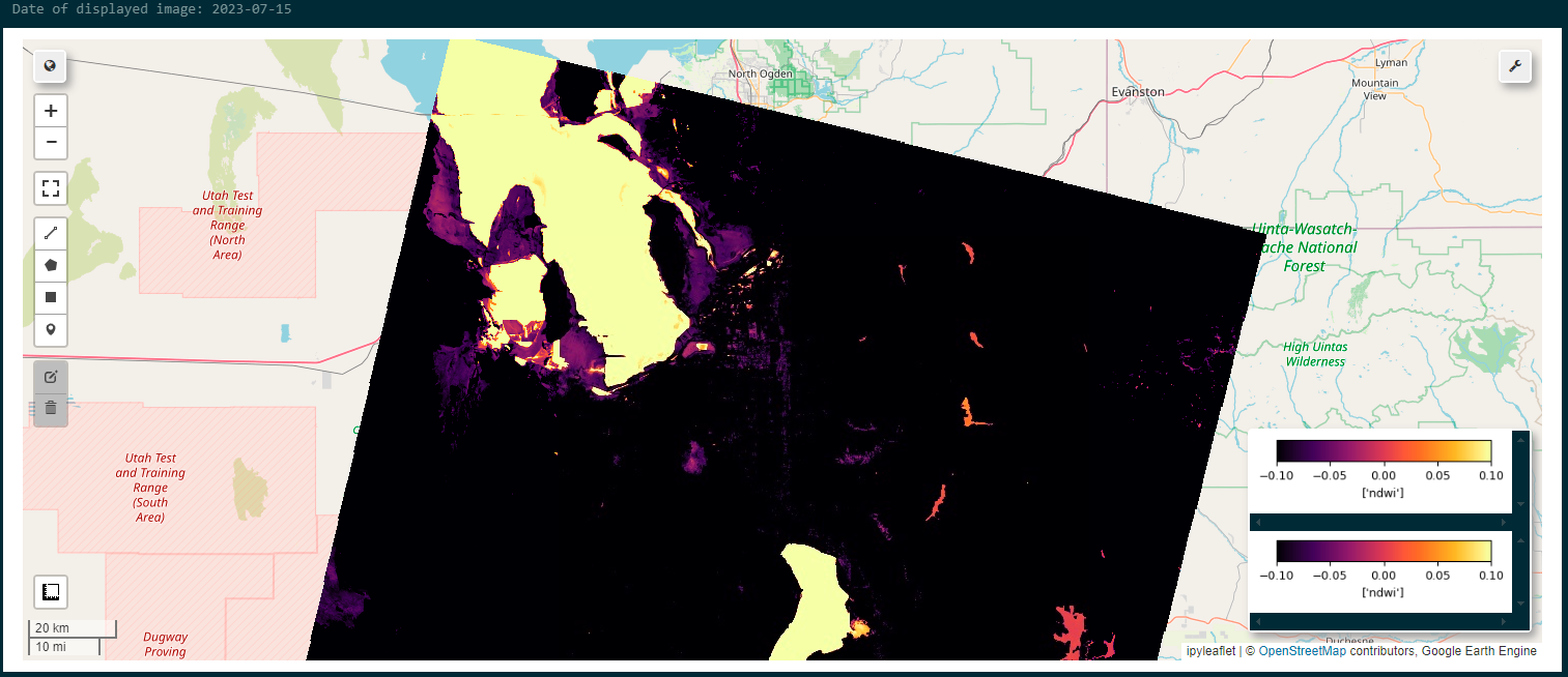
NDWI Visualization
[8]:
Map = geemap.Map(center=(40.7514, -111.9064), zoom=9)
# min and max values are optional but allow for customization
Map.addLayer(ndwi.image_grab(-1), vis_params=VisParams.get_visualization_params('Landsat', 'NDWI', min_val=-0.1, max_val=0.1))
Map.add_colorbar(vis_params=VisParams.get_visualization_params('Landsat', 'NDWI', min_val=-0.1, max_val=0.1))
print('Date of displayed image:', ndwi.dates[-1])
Map
Date of displayed image: 2023-07-15
[8]:
Example of NDWI Map Output from Above Cell
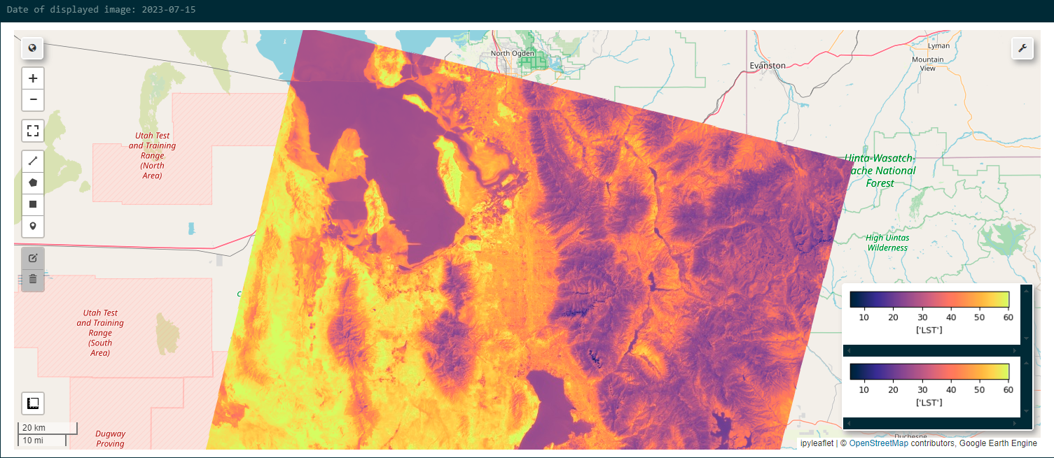
Land Surface Temperature Visualization
[9]:
Map = geemap.Map(center=(40.7514, -111.9064), zoom=9)
vis_params=VisParams.get_visualization_params('Landsat', 'LST', min_val=5, max_val=60)
Map.addLayer(LST.image_grab(-1), vis_params=vis_params)
Map.add_colorbar(vis_params=vis_params)
print('Date of displayed image:', LST.dates[-1])
Map
Date of displayed image: 2023-07-15
[9]:
Example of Land Surface Temperature Map Output from Above Cell
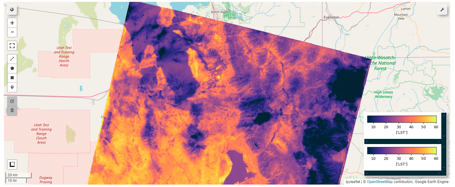
Mean LST image visualization
[10]:
Map = geemap.Map(center=(40.7514, -111.9064), zoom=9)
vis_params=VisParams.get_visualization_params('Landsat', 'LST', min_val=5, max_val=60)
Map.addLayer(mean_temperature, vis_params=vis_params)
Map.add_colorbar(vis_params=vis_params)
Map
[10]:
Example of Mean Land Surface Temperature Map Output from Above Cell
Finally, lets look at a chained example looking at turbidity in water pixels - but let’s do it taking full advantage of the package
Look how little code is needed to define the collection using multiple landsat tiles, mosaic images with the same date, mask the collection to water pixels, and calculate the relative turbidity of the water pixels - then display it!
Note the location and date are for demonstrative purposes only.
[11]:
masked_turbidity_col = LandsatCollection('2023-04-01', '2023-07-30', [32, 33], 38, 20).MosaicByDate.masked_to_water_collection.turbidity
image = masked_turbidity_col.image_grab(-1) #get latest image
When processing turbidity, the band name become ‘ndti’ for Normalized Difference Turbidity Index
[12]:
print('Band name of turbidity image: ', image.getInfo()['bands'][0]['id'])
Band name of turbidity image: ndti
Let’s see what it looks like on the map!
[13]:
Map = geemap.Map(center=(40.7514, -111.9064), zoom=9)
vis_params=VisParams.get_visualization_params('Landsat', 'NDTI')
Map.addLayer(image, vis_params=vis_params)
Map.add_colorbar(vis_params=vis_params)
Map
[13]:
Example of Turbidity Map Output from Above Cell
