S1 SAR Backscatter Basic Usage

Note:

This notebook includes interactive map visualizations using the geemap package. Additionally, you will likely need to install ipykernel to utilize the interactive elements within a Jupyter Notebook. The geemap and ipykernel packages are not installed automatically with RadGEEToolbox since they are optional dependencies focused on visualizations. If you have not already installed these packages, you can do so with:

pip install geemap ipykernel

Alternatively, using conda:

conda install conda-forge::geemap anaconda::ipykernel

If you do not install them, the map-based portions of this notebook will not work.

Initialization and Setup

import ee
from RadGEEToolbox import Sentinel1Collection

# Store name of Google Cloud Project assosiated with Earth Engine - replace with your project ID/name
PROJECT_ID = 'your-cloud-project-id'

# Attempt to initialize Earth Engine
try:
    ee.Initialize(project=PROJECT_ID)
    print("Earth Engine initialized successfully.")
except Exception as e:
    print("Initialization failed, attempting authentication...")
    try:
        ee.Authenticate()
        ee.Initialize(project=PROJECT_ID)
        print("Authentication and initialization successful.")
    except Exception as auth_error:
        print("Authentication failed. Error details:", auth_error)

Earth Engine initialized successfully.

Quickly defining an ROI for filtering imagery - can be any ee.Geometry()

Note: You may filter based on relative orbit numbers in addition to a geometry

# First we will define a region of interest (ROI) for the analysis, in this case, Salt Lake County, Utah.
counties = ee.FeatureCollection('TIGER/2018/Counties')
salt_lake_county = counties.filter(ee.Filter.And(
    ee.Filter.eq('NAME', 'Salt Lake'),
    ee.Filter.eq('STATEFP', '49')))
salt_lake_geometry = salt_lake_county.geometry()

---

Image collection definition and filtering

Define the desired parameters to initialize the Sentinel-1 SAR collection using the Sentinel1Collection() class.

In this case, filtering to dual-polarized (VV/VH) descending IW scenes during May of 2024

SAR_collection = Sentinel1Collection(
    start_date='2024-05-01',
    end_date='2024-05-31',
    instrument_mode='IW',
    polarization=['VV', 'VH'],
    orbit_direction='DESCENDING',
    boundary=salt_lake_geometry,
    resolution_meters=10
)

The image will be much larger than the boundary of the study area, so let’s mask the data using the salt_lake_geometry shape and .mask_to_polygon() to reduce processing time moving forward

SAR_collection = SAR_collection.mask_to_polygon(salt_lake_geometry)

Now let’s print the dates of the collection to validate

dates = SAR_collection.dates
print("SAR Collection Dates:", dates)

SAR Collection Dates: ['2024-05-04', '2024-05-04', '2024-05-11', '2024-05-11', '2024-05-23', '2024-05-23', '2024-05-28', '2024-05-28']

---

Multilooking and speckle filtering are very common workflows for SAR data, and ``RadGEEToolbox`` provides functionality for both

S1 SAR data hosted by GEE is in units of decibels (dB, logarithmic) but units of σ⁰ (backscatter coefficient, linear) are more suitable for multilooking and speckle filtering.

First, we convert from dB to σ⁰ using ``.sigma0FromDb``

SAR_collection_sigma0 = SAR_collection.sigma0FromDb

Then Perform Multilooking using ``.multilook()`` - in this case using 4 looks

SAR_collection_multilooked = SAR_collection_sigma0.multilook(looks=4)

Now perform speckle filtering on the multilooked collection using ``.speckle_filter()``

When speckle filtering you must provide the kernel size (odd integer between 3-9). You may optionally tweak the speckle filter process by adjusting the geometry used for windowed statistics, the Tk value, sigma value, and number of looks of the input collection.

In this case we choose a kernel size of 5x5, use the geometry of our ROI, and specify that the input collection is multilooked by 4 looks (important for the correct LUT usage)

SAR_collection_multilooked_and_filtered = SAR_collection_multilooked.speckle_filter(5, geometry=salt_lake_geometry, looks=4)

Print the dates of the multilooked and speckle filtered SAR collection using ``.dates`` to verify the filtering worked successfully

print(SAR_collection_multilooked_and_filtered.dates)

['2024-05-04', '2024-05-04', '2024-05-11', '2024-05-11', '2024-05-23', '2024-05-23', '2024-05-28', '2024-05-28']

Now we convert back to dB for analysis and visualization using ``.dbFromSigma0``

SAR_collection_multilooked_and_filtered_db = SAR_collection_multilooked_and_filtered.dbFromSigma0

---

Example of how to temporally reduce the results by processing a mean composite using ``.mean``

mean_SAR_image = SAR_collection_multilooked_and_filtered_db.mean

---

If you wish to visualize the results follow the code below. You will need to have the ``geemap`` package installed

import geemap
from RadGEEToolbox import GetPalette
from RadGEEToolbox import VisParams

Run the cell below to view the results on the map

Note: the raster is very detailed, so it may take a few seconds once done processing to display the image on the map

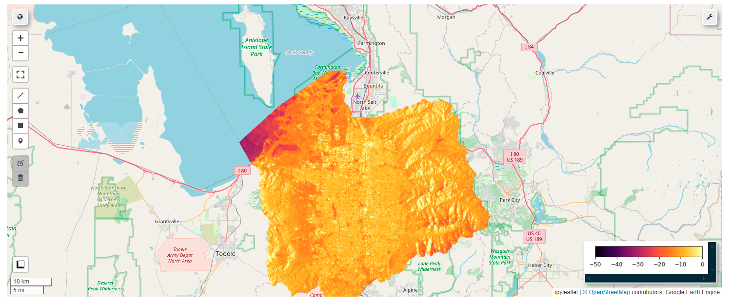
Map = geemap.Map(center=(40.7514, -111.9064), zoom=10)
Map.addLayer(mean_SAR_image.select('VV'), vis_params={'min': -50, 'max': 0, 'palette': GetPalette.get_palette('inferno')}, name='NDWI')
Map.add_colorbar(vis_params={'min': -50, 'max': 0, 'palette': GetPalette.get_palette('inferno')})
Map

Example of What Map Should Look Like

Please refer to theRadGEEToolbox documentationfor more information and a comprehensive list of available functionality